Particle Swarm Optimization(PSO) - UNIGOU academic collaboration

Description

In a collaborative project with Michal Bildo at Brno University in the Czech Republic, made possible by the UNIGOU program, I embarked on a journey to explore the world of Nature-Inspired Algorithms conducted by Michal, who guided my steps on this journey.

After a review of the literature and gaining insight into some of the principal nature-inspired algorithms, we decided to place a special emphasis on the Particle Swarm Optimization(PSO) technique. Our mission was to bring PSO to an educational graphical interface.

The softwares presented in this article were developed with the intention of offering students and teachers a chance to study, demonstrate, and visualize PSO; also allowing experimentation and personal adjustments. Here we bring two implementations of PSO: one to seek minima in 3D functions(simpler problem but with better visualization) and another to find best solutions to the complex Traveling Salesperson Problem(TSP).

Theory

PSO and its origin

PSO is a stochastic nature-inspired optimization method based on swarm, it was introduced by Eberhart and Kennedy in 1995. PSO mimics the collective behavior of some animals and is used to find optimal solutions to complex problems by iteratively adjusting a population of potential solutions based on their fitness. PSO can be applied to various domains, including the optimization of mathematical functions and solving combinatorial problems like the Traveling Salesperson Problem as we will see in the following.

As commented above, PSO draws its inspiration from natural phenomena, particularly the collective behavior of some animals like birds and fishes for example:

• Flocking Behavior of Birds: Birds in a flock exhibit coordinated movement, adjusting their positions based on the behavior of neighboring birds. This collective behavior helps the flock optimize its path and react to environmental changes.

• Schooling Behavior of Fish: Similar to birds, fish in a school demonstrate collective behavior in their underwater journeys. They move as a group, responding to the movements and cues of other fish. This synchronized behavior allows fish to find optimal routes and adapt to changing conditions in their aquatic environment.

In PSO, individual solutions represented as particles, explore a multidimensional search space while adjusting their positions based on the performance of other particles. This mimics the way birds, fishes and other animals collectively adapt and optimize their trajectories in response to their peers.

The beauty of PSO lies in its ability to translate these natural principles into an effective optimization technique, making it a valuable tool for solving complex problems across various domains and deepening our appreciation for nature.

Understanding PSO algorithm

PSO operates on the principles of swarm intelligence, and its key components include:

1. Particles: In PSO, each potential solution is represented as a particle in a search space. These particles explore the space to find the optimal solution.

2. Fitness Function: The fitness function is the metric for assessing the quality of a solution found by the particle during the exploration. It varies according to the problem.

3. Social Influence: Particles are influenced by the collective knowledge of the swarm. The social influence guides particles toward the global best solution. In general, this coefficient is responsible for the convergence of the algorithm.

4. Cognitive Influence: Each particle maintains its own historical best solution. The cognitive influence guides particles toward their individual best solutions.

5. Inertia Influence: The inertia weight balances the trade-off between global exploration and local exploitation. It helps particles regulate their movement within the search space.

An classical example of an equations to govern the particles movement in PSO are as follows:

• Velocity Update: The velocity of each particle is updated at each iteration based on its current velocity, cognitive influence, and social influence.

    v_i(t+1) = inertia_w * v_i(t) + cognitive_w * rand1 * (pBest_i - x_i(t)) + social_w * rand2 * (gBest - x_i(t))
  

  Where:

  • x_i(t) is the current position of particle i at time t.
  • v_i(t) is the current velocity of particle i at time t.
  • v_i(t+1) is the updated velocity of particle i at time t+1.
  • social_w is the social weight.
  • cognitive_w is the cognitive weight.
  • inertia_w is the inertia weight.
  • rand1 and rand2 are random values between 0 and 1.
  • pBest_i is the best-known position of particle i.
  • gBest is the global best-known position in the swarm.
• Position Update: The position of each particle is updated based on its velocity.

    x_i(t+1) = x_i(t) + v_i(t+1)
  

  • x_i(t+1) is the updated position of particle i at time t+1.

These equations govern the movement of particles within the search space, enabling PSO to search for optimal solutions through collective behavior and iterative adjustments.

To implement the PSO algorithm, as exemplified in the following examples, the key steps entail creating a pertinent set of particles and fitness function to represent the problem. Then, it is just keep updating the particles’ positions and evaluating their fitness values iterativelly in accordance with the equations mentioned above(or suitable adaptations), until the algorithm converges or completes a predefined number of iterations.

Practice

Finding Minimum of 3D Functions

In this example, we utilize PSO to discover the minimum of 3D functions. The implementation can be found here: PSO-min-3d-functions. Feel free to customize the code as needed. The user interface is designed to accommodate various parameter variations. Bellow you can see a gif demostrating it in action.

Input:

• Select a predefined function from a range of classical optimization functions based on this list.
• Input your custom function, following the Python w/numpy format as demonstrated in the following example: np.cos(np.sqrt(x**2 + y**2))*(x+y).
• Define the function range on the X and Y axes.
• Define the number of particles.
• Define the number of iterations.
• Set the inertia weight.
• Set the cognitive weight.
• Set the social weight.
• Set the initial velocity in the X-axis.
• Set the initial velocity in the Y-axis.

Output:

• The best solution found.
• The execution time.
• The animation of particles reaching the result(essential for the educational aspect).

About the Code

The code is structured into three simple components:

main.py

• TkInter UI: Responsible for creating the user interface using TkInter. It allows users to interact with the PSO algorithm and set various parameters.
• Animation: It includes methods for visualizing the PSO process.
• Integration: Connects the inputs of the UI to the other components and present the results provided by the other components to the TkInter UI.

particle.py

• Particle Definition: This module defines the properties and behavior of individual particles used in the PSO algorithm to find the minimum of a 3d function.

pso.py

• PSO Algorithm: This module contains the PSO algorithm implementation.

To start it, run “python3 main.py”. To get more details about the implementation, please visit the source code. If you have any questions or suggestions, feel free to contact me.

Suggested Reflections

While exploring this interface, if this is your first interaction with PSO and you haven’t quite grasped how it works yet, try adjusting the parameters to observe its behavior and consider the following questions:

• How would you define the cognitive weight in one word based on what it represents to the algorithm?
• How would you define the social weight in one word based on what it represents to the algorithm?
• What occurs when you set the cognitive weight to 0?
• What occurs when you set the social weight to 0?
• What occurs when you set the inertia weight to 0?
• What happens when you significantly increase the number of particles?
• What happens if you set an exceptionally high initial velocity?
• Do parameters that perform well with one type of function also perform well with all other functions?
• What about making parameters(weights) vary over iteractions in accordance and specific function or behavior? Can you imagine how this can improve the performance of the algorithm?

Conducting experiments and contemplating this kind of questions can help you understanding the concept of PSO.

Traveling Salesperson Problem(TSP)

TSP is a combinatorial optimization problem where the goal is to find the shortest possible route that visits a predefined set of given cities exactly once, while minimizing the total distance traveled. In other words, it asks for an optimal sequence in which a traveling salesperson should visit a series of cities to minimize the total distance traveled in the end. This problem has practical applications in various fields, such as logistics, transportation, circuit design and others.

For example, consider the task of finding the optimal route that passes through all of Brazil’s state capitals, as ilustrated in the map below. This is a possible instance of the TSP problem, where the objective is to identify the path that visits all capitals while minimizing the overall distance cost.

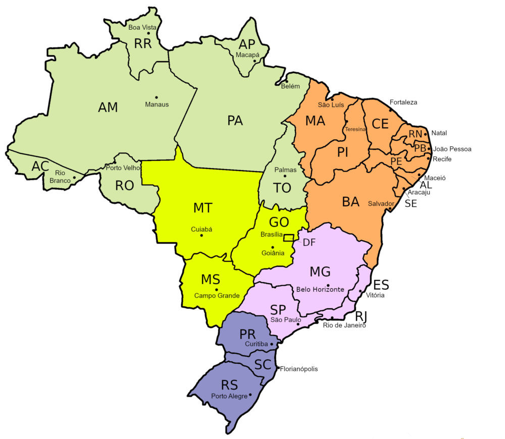
Just out of curiosity, the optimal solution for the TSP covering Brazil’s state capitals is as follows: Belo Horizonte -> Goiânia -> Brasília -> Palmas -> Salvador -> Aracaju -> Maceió -> Recife -> João Pessoa -> Natal -> Fortaleza -> Teresina -> São Luís -> Belém -> Macapá -> Boa Vista -> Manaus -> Porto Velho -> Rio Branco -> Cuiabá -> Campo Grande -> Porto Alegre -> Florianópolis -> Curitiba -> São Paulo -> Rio de Janeiro -> Vitória. So, if you ever plan to one day visit all the state capitals in Brazil, I strongly recommend following this order to minimize fuel consumption - hehehe

Now let’s talk about our implementation. In this example, we utilize PSO to try discovering the best route through N random cities positioned in the 2d space. The implementation can be found here: PSO-tsp. Feel free to customize the code as needed. The user interface is designed to accommodate parameter variations and output the results as graph and logs. Bellow you can see a gif demostrating it in action.

Input:

• Number of cities.
• Cities disposition on the map: random or in a circle. The circle layout can be especially useful as it provides an intuitive best solution, making it easier to visually assess algorithm performance.
• Specify the number of particles.
• Set the number of iterations.
• Define the cognitive weight.
• Define the social weight.
• Optionally, add a greedy particle (useful in some situations, not in others).

Note: The sum of the cognitive weight + social weight + inertia weight must equal 1 in this implementation, which is why there is no separate field for inertia weight in this version; it is implicit.

Output:

• The top 5 solutions found.
• A convergence graph.
• Detailed logs with the entire history of all particles for analysis.

About the Code

The code is structured into three simple components:

main.py

• Initiates the GTK UI.

tsp.py

• Problem Definition: This module defines the problem instance and includes helpful methods for tasks like city generation, arranging them in a circle, and other relevant functions specially for the UI.

pso.py

• PSO Algorithm: This module encompasses the implementation of the PSO algorithm. It defines particles and cities and forms the core logic of the project.

FileWriter.py

• Machanism to log: Responsible for logging all algorithm iterations for subsequent analysis inside the /data directory.

gui

• A module containing the graphical interface implemented in GTK, with the following subcomponents:
• psoparams.py: Maps the widget states to mainwindow.py.
• solviewer.py: Manages the display area for cities and showcases new best paths upon request of mainwindow.py and things like that.
• mainwindow.py: Responsible to get the parameters from psoparams.py, execute the algorithm and update the UI of solviewer.py when necessary.

To start it, run “python3 main.py” inside the “src” directory. For more detailed information about the implementation, please visit the source code. If you have any questions or suggestions, don’t hesitate to reach out to me.

Suggested Reflections

• A great exercise, once you’ve thoroughly grasped the first example involving 3d functions, is to contemplate how to update the state of a particle in the TSP case. After giving it some thought, exploring the source code to see the implemented approach, how can we improve this method of updating the particles?

• Another intriguing aspect to ponder is whether there exists a fundamental distinction between the 3d function example and the TSP beyond the dimensionality of the problems. In other words, is there a K-dimensional version of the initial function minimization problem that can fit any instance of TSP with X cities? And if such a version exists, what would be the minimum number of dimensions K for X cities? Does the dimensions really make any difference one time that the functions are in theory continous(even 2d functions)?

• Are there any better ways to visualize PSO for TSP than showing the best solution? Is there a good way to map a instance of TSP solution for X cities in a 2d, 3d or even 4d(with colors) space for a better visualization?

Some of these questions have well-defined answers, but it is important to remember that the journey to finding those answers often holds more value than the answers themselves - so, try thinking by yourself!!! - Other questions continue to intrigue me. Anyway, the true joy lies in the process of exploration and learning - embracing the mysteries and challenges that come along the way. Keep the curiosity alive!

Notes about the educational interface development

One of my responsibilities during this academic collaboration was to create an educational interface aimed at helping people to grasp the concepts of PSO and its practical application in solving the TSP.

While implementing the TSP interface, I faced a significant challenge in creating a didactic visualization method for illustrating the TSP problem being solved by PSO. After much exploration, I found that the most effective representation was to showcase the evolving best route as found by the current best particle - I believe that exists better approaches, but I was not able to discover them yet. Given TSP’s complexity as an optimization problem, it presents challenges in its visual representation.

To provide a more didactic approach and address a problem with greater visualization potential, I also designed an interface for locating minimum points within three-dimensional functions using PSO. This interface features a variety of classical optimization functions for straightforward testing and enables users to input their own custom functions for experimentation, I believe it is a better starting point than TSP for begginers in PSO.

Conclusion

Thank you for reading this far. This post is intended to introduce PSO and showcase the interfaces were developed in this project for educational purposes. If you have any questions or suggestions, please don’t hesitate to reach out to me.

Certificate

Certificate

Assesment letter